An introduction to gradient descent algorithms

Moulay Abdellah CHKIFA
April 29-30, 2019
Faculty of Sciences and Techniques (FST), Mohammedia
Linear Regression
Principle
Linear regression algorithms are used for prediction purposes. An affine linear model makes a prediction by simply computing a weighted sum of the input features, plus a constant called the bias term (or intercept term)
\begin{equation} \hat y = \theta_0 +\theta_1 x_1 +\theta_2 x_2 +\dots+ \theta_n x_n = \theta \cdot {\bf x} = h_\theta({\bf x}). \end{equation}where $$ \theta := (\theta_0,\dots,\theta_n)^T, \quad\quad {\bf x}:=(x_0,x_1,\dots,x_n)^T,\quad x_0=1. $$
- $n$ is the number of features.
- $x_i$ is the $i^{th}$ feature value.
- $h_\theta$ is the hypothesis function, using the model parameters $\theta$.
- $\hat y$ is the predicted value.
Loss function
The MSE of hypothesis $h_\theta$ on a training set $\{(x^{(1)},y^{(1)}),\dots,(x^{(m)},y^{(m)})\} \subset \mathbb R^n \times \mathbb R$ is given by \begin{equation} J(\theta) = MSE(X,h_\theta) = \frac 1{m} \sum_{i=1}^m ( h_\theta({\bf x}^{(i)}) - y^{(i)} )^2 \end{equation}
Gradient computation
We have $\nabla J(\theta):= \big(\frac{\partial J}{\partial \theta_0}(\theta),\dots \frac{\partial J}{\partial \theta_n}(\theta) \big)^T$ and the partial derivative of $J$ with respect to $\theta_j$ is
\begin{equation} \frac{\partial J}{\partial \theta_j}(\theta)=\frac 1m\sum_{i=1}^m 2 x_j^{(i)} ( h_\theta({\bf x}^{(i)}) - y^{(i)} ) \end{equation}We have \begin{equation} \nabla J(\theta):= \frac 1m 2 X^T (X\theta - Y) \end{equation}
Batch gradient descent
The Batch gradient descent algorithm is given by
\begin{equation} \theta^{(0)} \mbox{ initial guess},\quad \quad\quad \theta^{(k+1)}= \theta^{(k)} - \eta \nabla J(\theta^{(k)}) \end{equation}The whole batch $X$ of training data is used at every step.
The loss function is quadratic in $\theta$ (hence convex) and clearly L-smooth with
$$ L=\frac 2m\|X^{T}X\|_{2\to2}= \frac 2m s_1(X)^2 $$where $s_1(X)$ is the largest singular value of $X$. Batch gradient descent with learning rate $\eta<1/L$ converge to $\theta^*$ which minimizes $J$.
Solving normal equation $(y=2+5x+\mbox{noise})$
## Direct computation using normal equation
%matplotlib inline
import numpy as np
import matplotlib.pyplot as plt
n,m = 1,200
x = 2* np.random.rand(m, n)
y = 2 + 5 * x + 0.5* np.random.randn(m, n) ## thus theta0= 2 , theta1=5
plt.scatter(x, y)
X_b = np.c_[np.ones((m, n)), x] # add x0 = 1 to each instance
theta_best = np.linalg.inv(X_b.T.dot(X_b)).dot(X_b.T).dot(y)
plt.plot([0,2],[theta_best[0],theta_best[0]+2*theta_best[1]],color='r')
print ('theta_best=',theta_best)
plt.show()

Gradient descent for $(y=2+5x+\mbox{noise})$
## gradient descent applied to the function J: theta -> J (theta) ##
def val_f (theta):
return (1./m)*np.linalg.norm(X_b.dot(theta) - y)
def grad_f (theta):
return (2./m)*X_b.T.dot(X_b.dot(theta) - y)
x0 = np.zeros((2, 1))      # The algorithm starts at x0=(0,0)

s1 = np.linalg.norm(X_b, ord=2) ## Largest singular value of X_b
L = (2/m)*s1*s1            # L for L-smoothness
rate = 1./L                # Learning rate
precision = 0.001          # This tells us when to stop the algorithm
step_size = 1              # step being taken
max_iters = 4000           # maximum number of iterations
iters = 0                  #iteration counter

vec_x,vec_f  = [],[]
cur_x = x0
while step_size > precision and iters < max_iters:
vec_x = vec_x+[cur_x]
vec_f = vec_f+[val_f(cur_x)]
prev_x = cur_x                        #Store current x value in prev_x
cur_x = cur_x - rate * grad_f(prev_x) #Gradien descent
step_size = np.linalg.norm(cur_x - prev_x)   #Change in x
iters = iters+1 #iteration count
print("The local minimum occurs at", vec_x[-1])
print("The local minimum is equal to", vec_f[-1])
Gradient descent visualised
## Animation based on gradient descent applied for linear regression ##

import numpy as np
from matplotlib import pyplot as plt
from matplotlib.pyplot import figure
from matplotlib import animation, rc

#%matplotlib inline
#matplotlib notebook
#%matplotlib nbagg
%matplotlib tk

# First set up the figure, the axis, and the plot element we want to animate

fig = plt.figure()
fig.set_dpi(100)

xmin,xmax = 0, 2
fmin,fmax = 1,14

ax  = plt.axes(xlim=(xmin, xmax), ylim=(fmin, fmax))
line, = ax.plot([], [], lw=2,color='r')

# initialization function: plot the background of each frame
def init():
plt.scatter(x, y,color='b')
line.set_data([], [])
return line,

# animation function.  This is called sequentially
def animate(i):
a = [0,2]
theta= vec_x[i]
b = [theta[0],theta[0]+2*theta[1]]
line.set_data(a, b)
return line,

# call the animator.  blit=True means only re-draw the parts that have changed.
anim = animation.FuncAnimation(fig,
animate,
init_func=init,
frames=50,
interval=50,
blit=True)

# save the animation as an mp4.  This requires ffmpeg or mencoder to be
# installed.  The extra_args ensure that the x264 codec is used, so that
# the video can be embedded in html5.  You may need to adjust this for
# your system: for more information, see
# http://matplotlib.sourceforge.net/api/animation_api.html

#HTML(anim.to_html5_video())

from IPython.display import HTML
anim.save('GD_converge.mp4', fps=5, extra_args=['-vcodec', 'h264', '-pix_fmt', 'yuv420p'])
plt.show()
Variants: interpretability, etc
- Lasso regression $$ J(\theta) = \frac 1m \|X\theta-Y\|^2 + \lambda \|\theta\|_1 $$
- Ridge regression $$ J(\theta) = \frac 1m \|X\theta-Y\|^2 + \|\Gamma \theta\|^2 $$
Stochastic Gradient Descent
Principle
We are interested in minimizing the additive loss function
\begin{equation} J(\theta) = \sum_{i=1}^m J_i(\theta),\quad\quad\quad J_i(\theta):= ( h_\theta({\bf x}^{(i)}) - y^{(i)} )^2 \end{equation}One random instance $\{(x^{(\omega)},y^{(\omega)})\}$ in the training set is picked at every step $k$ and the gradient is computed based only on this instance. This gradient is $\nabla J_\omega(\theta) = \nabla_\theta J_\omega(\theta)$ and is equal to
\begin{equation} \nabla J_\omega(\theta):= 2 (h_\theta({\bf x}^{(\omega)}) - y^{(\omega)}) {\bf x}^{(\omega)}. \end{equation}The Stochastic Gradient Descent (SGD) algorithm for MSE minimization in linear regression is given by
\begin{equation} \theta^{(0)} \mbox{ initial guess},\quad \quad\quad \left\{\begin{array}{} {\omega} \mbox{ randomly selected in} \{1,2,\dots,m\} \\ \theta^{(k+1)}= \theta^{(k)} - \eta \nabla J_{\omega}(\theta^{(k)}) \end{array} \right. \quad\quad\quad k\geq0. \end{equation}Only one random instance $\{(x^{(\omega)},y^{(\omega)})\}$ of training data $X$ is used at every step.
- Every step $k$ of the algorithm is much faster.
- This makes it possible to train on large training sets.
n_epochs = 50
t0, t1 = 5, 50 # learning schedule hyperparameters
def learning_schedule(t):
return t0/(t+t1)

theta = np.random.randn(2,1) # random initialization
for epoch in range(n_epochs):
for i in range(m):
random_index = np.random.randint(m)
xi = X_b[random_index:random_index+1]
yi = y[random_index:random_index+1]
gradients = 2 * xi.T.dot(xi.dot(theta) - yi)
eta = learning_schedule(epoch * m + i)
theta = theta - eta * gradients

print(theta)
Using SGDRegressor
from sklearn.linear_model import SGDRegressor
sgd_reg = SGDRegressor(n_iter=50, penalty=None, eta0=0.1)
sgd_reg.fit(x, y.ravel())
sgd_reg.intercept_, sgd_reg.coef_
Variant
- Mini-batch SGD
- Momentum
- Nesterov accelerated gradient
- Adagrad / Adadelta / RMSprop / Adam / AdaMax / Nadam
from IPython.display import IFrame
IFrame(src='https://arxiv.org/pdf/1609.04747.pdf', width=700, height=600)
Logistic Regression
Principle
Logistic Regression (also called Logit Regression) algorithms are used for binary classification. The model estimates the probability that an instance belongs to one of two classes ({0,1} or {Y,N} or {+,-} etc) and predicts for the instance the class with the highest probability.
For classes $y$ in $\{0,1\}$, the model estimate a parameter $\theta= (\theta_0,\theta_1,\dots,\theta_n)^T\in {\mathbb R}^{n+1}$ and classifies (i.e. predicts the class) according to
\begin{equation} \hat y = \left\{ \begin{array}{cc} 0 \quad \mbox{if}\quad \sigma(\theta.{\bf x})<0.5 \\ 1 \quad \mbox{if}\quad \sigma(\theta.{\bf x})\geq 0.5 \end{array} \right. \end{equation}where $\sigma$ is the sigmoid function.
Logistic function

Observe:
● $\sigma(\theta\cdot{\bf x})\lt0.5$ if and only if $\theta \cdot {\bf x} \lt 0$.
Observe:
\begin{equation}
\sigma'(t) = \sigma(t) (1- \sigma(t))
\end{equation}
Loss function
Here $\hat p=\sigma(\theta. {\bf x})$ and we introduce the misslasification error
\begin{equation} c(\theta)=\left\{\begin{array}{l}- \log(\hat p)\quad &\quad y=1\\- \log(1- \hat p)\quad &\quad y=0\\ \end{array} \right. \quad\quad \equiv \quad\quad c(\theta) =-\bigg[\log(\hat p) y+ \log(1- \hat p) (1-y)\bigg] \end{equation}This error is intuitive
$-\log(\hat p)=\log(1/{\hat p})$ grows very large when $\hat p$ approaches $0$. The loss (or penalty) is large if the model estimates a probability close to $0$ for instance in class $1$.
$-\log(1-\hat p)$ is close to $0$ when $\hat p$ approaches $0$. The loss (or penalty) is small if the model estimates a probability close to $0$ for instance in class $0$. (Same observations if $\hat p$ approaches $1$).
Given a training set $\{(x^{(1)},y^{(1)}),\dots,(x^{(m)},y^{(m)})\} \subset \mathbb R^n \times \mathbb \{0,1\}$, the loss function is given by
\begin{equation} J(\theta) = \frac 1{m} \sum_{i=1}^m c^{(i)}(\theta),\quad\quad\quad c^{(i)}(\theta)=-\bigg[\log(\hat p^{(i)}) y^{(i)} + \log(1- \hat p^{(i)}) (1-y^{(i)})\bigg] \end{equation}Gradient computation
Given $c(\theta) =-\big[\log(\hat p) y+ \log(1- \hat p) (1-y)\big]$, observe $$ \frac {\partial c }{\partial \theta_j} =\frac {\partial c }{\partial \hat p }\frac {\partial \hat p }{\partial (\theta.{\bf x})}\frac {\partial (\theta.{\bf x})}{\partial \theta_j } =\frac {\partial c }{\partial \hat p }\;\sigma'(\theta.{\bf x})\;x_j $$ We have $$ \frac {\partial c }{\partial \hat p } = -\bigg[\frac 1 {\hat p} y - \frac 1{1- \hat p} (1-y)\bigg]\quad\quad\sigma'(\theta.{\bf x})\;= \sigma (\theta.{\bf x}) (1-\sigma(\theta.{\bf x})) = \hat p (1- \hat p) $$ Finally $$ \frac {\partial c }{\partial \theta_j}=-\bigg[(1- \hat p) y - \hat p (1-y)\bigg]x_j=\big[ \hat p -y \big]x_j $$
The partial derivatives of $J$ are given by \begin{equation} \frac {\partial J(\theta) }{\partial \theta_j}=\frac 1{m} \sum_{i=1}^m \frac {\partial c^{(i)}(\theta) }{\partial \theta_j}=\frac 1{m} \sum_{i=1}^m \big[ \sigma(\theta.{\bf x}^{(i)})-y^{(i)} \big]\;x_j^{(i)} \end{equation}
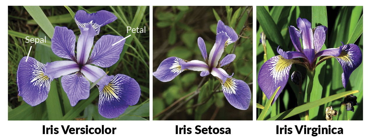
Decision Boundaries for the iris flower dataset
from sklearn import datasets
iris = datasets.load_iris()
list(iris.keys())
iris['feature_names']
from sklearn.linear_model import LogisticRegression

X = iris["data"][:, (2, 3)]  # petal length, petal width
y = (iris["target"] == 2).astype(np.int)

log_reg = LogisticRegression(C=10**10, random_state=42)
log_reg.fit(X, y)

x0, x1 = np.meshgrid(np.linspace(2.9, 7, 500).reshape(-1, 1),
np.linspace(0.8, 2.7, 200).reshape(-1, 1),)
X_new = np.c_[x0.ravel(), x1.ravel()]

y_proba = log_reg.predict_proba(X_new)

plt.figure(figsize=(10, 4))
plt.plot(X[y==0, 0], X[y==0, 1], "bs")
plt.plot(X[y==1, 0], X[y==1, 1], "g^")

zz = y_proba[:, 1].reshape(x0.shape)
contour = plt.contour(x0, x1, zz, cmap=plt.cm.brg)


left_right = np.array([2.9, 7])
boundary = -(log_reg.coef_[0][0] * left_right + log_reg.intercept_[0]) / log_reg.coef_[0][1]

plt.clabel(contour, inline=1, fontsize=12)
plt.plot(left_right, boundary, "k--", linewidth=3)
plt.text(3.5, 1.5, "Not Iris-Virginica", fontsize=14, color="b", ha="center")
plt.text(6.5, 2.3, "Iris-Virginica", fontsize=14, color="g", ha="center")
plt.xlabel("Petal length", fontsize=14)
plt.ylabel("Petal width", fontsize=14)
plt.axis([2.9, 7, 0.8, 2.7])
save_fig("logistic_regression_contour_plot")
plt.show()

Softmax regression
Principle
Softmax regression generalizes logistic regression in order to support $K$ classes. The model estimates a parameter matrix
\begin{equation} \Theta = [\Theta_1|\Theta_2\dots|\Theta_K]^T\in {\mathbb R}^{K \times (n+1)},\quad\quad \Theta_k =(\Theta_{0,k},\Theta_{1,k},\dots,\Theta_{n,k} )^{T}. \end{equation}Given $x\in{\mathbb R}^n$ and ${\bf x} = (1,x) \in {\mathbb R}^{n+1}$, we compute $z=\Theta {\bf x}~$ ( i.e. $z_j=\Theta_j. {\bf x}$ for every $j=1,\dots,K$), then compute the $K$ probabilities
\begin{equation} \hat p_k = \frac {\exp({z_k})}{\displaystyle\sum_{j=0}^K \exp({z_j})},\quad\quad k=1,\dots,K. \label{hatp_softmax} \end{equation}Example: Decision Boundaries for the iris flower dataset

Loss function
Here $\hat p$ is as in \eqref{hatp_softmax} and we introduce the misslasification error for $(x,y)$ by
\begin{equation} c(\Theta)= - \log (\hat p_k), \quad\quad \mbox{if}\quad\quad y = k. \end{equation}Intuitively, given $(x,y)$ with $y$ belongs to class $k$
- we want $c(\Theta)$ to be close to $0$, implying $\hat p_k$ close to $1$ (so that $\hat p_k$ is the highest probability).
- the closer $\hat p_k$ is to $0$ (i.e. the more certain that a miss-classification occurs), the larger is the loss (penalization) $c(\Theta)$.
Given a training set $\{(x^{(1)},y^{(1)}),\dots,(x^{(m)},y^{(m)})\} \subset \mathbb R^n \times \mathbb \{1,2,\dots,K\}$, the loss function is given by
$$ J(\Theta)= \frac 1{m} \sum_{i=1}^m c^{(i)}(\Theta)=- \frac 1{m} \sum_{i=1}^m \log (\hat p_{y^{(i)}}^{(i)}). $$Gradient computation
We let $\theta = \Theta_{j} \in \mathbb R^{n+1}$ for some $j\in \{1,\dots,K\}$: we have the following function dependency diagram
$$ \Theta \longrightarrow (z^{(i)}_l)_{\substack{i=1,\dots,m\\l=1,\dots,K}} \longrightarrow J. $$Using chain rule with respect to these intermediates variables and $\nabla_{\theta} z_l = \delta_{j,l}{\bf x}$ which follows from $z_l=\Theta_l. {\bf x}$,
$$\nabla_{\theta} J(\Theta)=\sum_{i=1}^m \sum_{l=1}^K\frac {\partial J(\Theta)}{\partial z_l^{(i)}}\nabla_{\theta} z_l^{(i)}=\sum_{i=1}^m \frac {\partial J(\Theta)}{\partial z_j^{(i)}}{\bf x}^{(i)}$$In view of the formula for $J$, for $i$ such that $y^{(i)}=k$ holds
$$ \frac {\partial J(\Theta)}{\partial z_j^{(i)}}= -\frac 1m \frac {\partial \log(\hat p_k^{(i)})}{\partial z_j^{(i)}} $$By derivation of usual functions, one has
$$\frac {\partial \log(\hat p_k)}{\partial z_j} =\frac 1{\hat p_k} \frac {\partial \hat p_k}{\partial z_j} = \frac 1{\hat p_k} \left\{ \begin{array}{ll} \hat p_k - (\hat p_k)^2&\quad \mbox{if}\quad j=k \\ - \hat p_k \hat p_j &\quad \mbox{if}\quad j\neq k \end{array} \right. = \left\{ \begin{array}{ll} 1 - \hat p_k&\quad \mbox{if}\quad j=k \\ - \hat p_j &\quad \mbox{if}\quad j\neq k \end{array} \right. $$The combination of the previous formulas implies that $J$ as a function of $(\Theta_1,\Theta_2,\dots,\Theta_K)$ satisfies
$$ \nabla_{\Theta_j} J(\Theta) = - \frac 1m \sum_{i=1}^m ({\mathbb 1}_{y^{(i)}=j} - \hat p_j^{(i)}) {\bf x}^{(i)} \quad\quad\quad\quad \nabla_{\Theta_j} J(\Theta) \in {\mathbb R}^{n+1}. $$Finally
$$ \nabla_{\Theta} J(\Theta) = [\nabla_{\Theta_1} J(\Theta) |\nabla_{\Theta_2} J(\Theta) |\dots|\nabla_{\Theta_k} J(\Theta) ]^T\in {\mathbb R}^{K \times (n+1)}. $$- Batch gradient descent;
- stochastic gradient descent;
- mini-Batch stochastic gradient descent;
can all be implemented.
X = iris["data"][:, (2, 3)]  # petal length, petal width, mainly for visualisation
y = iris["target"]

softmax_reg = LogisticRegression(multi_class="multinomial",solver="lbfgs", C=10, random_state=42)
softmax_reg.fit(X, y)
#lbfgs: Limited-memory Broyden–Fletcher–Goldfarb–Shanno algorithm.

x0, x1 = np.meshgrid( np.linspace(0, 8, 500).reshape(-1, 1),
np.linspace(0, 3.5, 200).reshape(-1, 1),)
X_new = np.c_[x0.ravel(), x1.ravel()]

y_proba = softmax_reg.predict_proba(X_new)
y_predict = softmax_reg.predict(X_new)

zz1 = y_proba[:, 1].reshape(x0.shape)
zz = y_predict.reshape(x0.shape)

plt.figure(figsize=(10, 4))
plt.plot(X[y==2, 0], X[y==2, 1], "g^", label="Iris-Virginica")
plt.plot(X[y==1, 0], X[y==1, 1], "bs", label="Iris-Versicolor")
plt.plot(X[y==0, 0], X[y==0, 1], "yo", label="Iris-Setosa")

from matplotlib.colors import ListedColormap
custom_cmap = ListedColormap(['#fafab0','#9898ff','#a0faa0'])

plt.contourf(x0, x1, zz, cmap=custom_cmap)
contour = plt.contour(x0, x1, zz1, cmap=plt.cm.brg)
plt.clabel(contour, inline=1, fontsize=12)
plt.xlabel("Petal length", fontsize=14)
plt.ylabel("Petal width", fontsize=14)
plt.legend(loc="center left", fontsize=14)
plt.axis([0, 7, 0, 3.5])
save_fig("softmax_regression_contour_plot")
plt.show()

Summary
How do we learn the "best" weights vector $(\theta_0^*,\dots,\theta_n^*)$ or matrix $(\Theta_0^*|\dots|\Theta_n^*)$ in linear/logistic/softmax regression
- Give weights random initial values
- Evaluate partial derivative of each weight with respect to MSE or negative log-likelihood at current weight value
- Take a step in direction opposite to the gradient
- Rinse and repeat

Neural network and backpropagation
MULTILAYER PERCEPTRONS (MLPs)

- Most generic form of a neural net is the "multilayer perceptron"
- Input undergoes a series of nonlinear transformation
- A final classification layer
- MLPs are easy entry to understand deep learning models
- Closely related to logistic/softmax regression
Principle
We consider classification problem for iris dataset using neural network with one hidden layer (5 nodes)
and activation function $\varphi$ (sigmoid, ReLU, etc)

- Input layer
$$x=(x_1,x_2,x_3,x_4)^T.$$- Hidden layer
$$h = (h_1,h_2,h_3, h_4,h_5)^T.$$- Output layer
$$z = ( z_1, z_2, z_3)^T.$$With bias in input and hidden layer $x_0 = 1, h_0=1$, we denote
$$ {\bf x} = (1,x^T)^T,\quad\quad\quad {\bf h} = (1,h^T)^T $$Neural network architechture

Artificial neurons

Loss function
As for softmax regression, the model minimizes the negative log-likelihood loss function associated with the training set $\{(x^{(1)},y^{(1)}),\dots,(x^{(m)},y^{(m)})\} \subset \mathbb R^n \times \mathbb \{1,2,\dots,K\}$ ($n=4$ and $K=3$ for iris dataset)
$$ J(\widetilde\Theta,\Theta) = - \frac 1{m} \sum_{{i=1}}^m \log (\hat p_k^{(i)}),\quad\quad\quad (k \mbox{ is such that } y^{(i)} \mbox{ belongs to class } k), $$in order to find the best parameter matrices $\widetilde\Theta^*$ and $\Theta^*$.
If $n_h$ is the number of nodes in the hidden layer (here $n_h=5$), we write
$$ \widetilde\Theta = [\widetilde\Theta_1|\widetilde\Theta_2\dots|\widetilde\Theta_{n_h}]^T\in {\mathbb R}^{n_h \times (n+1)},\quad\quad \Theta = [\Theta_1|\Theta_2\dots|\Theta_K]^T\in {\mathbb R}^{K \times (n_h+1)},\quad\quad $$
Gradients computation
We recall the mapping diagram
$$ {\bf x} \quad\Longrightarrow\quad h^{-} = \widetilde \Theta {\bf x} \quad\Longrightarrow\quad h = \varphi(h^{-}) \quad\Longrightarrow\quad z=\Theta {\bf h} $$and the function dependency diagram
$$ (\widetilde \Theta, \Theta) \longrightarrow ({h^{-}_j}^{(i)})_{\substack{i=1,\dots,m\\j=1,\dots,n_h}} \longrightarrow ({h_j}^{(i)})_{\substack{i=1,\dots,m\\j=1,\dots,n_h}} \longrightarrow (z^{(i)}_l)_{\substack{i=1,\dots,m\\l=1,\dots,K}} \longrightarrow J. $$- For $j=1,\dots,K$, we proceed as in soft-max regression (but as if $h$ is the input)
$$\nabla_{\Theta_j} J =\sum_{i=1}^m \frac {\partial J}{\partial z_j^{(i)}}{\bf h}^{(i)} = - \frac 1m \sum_{i=1}^m ({\mathbb 1}_{y^{(i)}=j} - \hat p_j^{(i)}) {\bf h}^{(i)}. $$Observe dependance on $\widetilde\Theta$ through the ${\bf h}^{(i)}$ then on $\Theta$ through the $\hat p_k^{(i)}$.
- For $j = 1,\dots,n_h$ and $\tilde\theta = \widetilde\Theta_{j}$, we proceed as in softmax regression: chain rule with variables $({h_l^{-}}^{(i)})_{\substack{i=1,\dots,m\\l=1,\dots,n_h}}$ and $h^{-} = \widetilde \Theta {\bf x}$ implies
$$\nabla_{\tilde\theta} J= \sum_{i=1}^m \sum_{l=1}^{n_h}\frac {\partial J}{\partial {h_l^{-}}^{(i)}} \nabla_{\tilde\theta} {h_l^{-}}^{(i)}= \sum_{i=1}^m \frac {\partial J}{\partial {h_j^{-}}^{(i)}} {\bf x}^{(i)}. $$Then $\frac {\partial J}{\partial {h_j^{-}}^{(i)}} =\frac {\partial J}{\partial h_j^{(i)}} \varphi'({h_j^{-}}^{(i)})$ and
$$ \frac {\partial J}{\partial h_j^{(i)}} = \sum_{l=1}^K \frac {\partial J}{\partial z_l^{(i)}} \frac {\partial z_l^{(i)}}{\partial h_j^{(i)}} = \sum_{l=1}^K \frac {\partial J}{\partial z_l^{(i)}} \Theta_{j,l}. $$The gradients $\nabla_{\Theta} J$ and $\nabla_{\widetilde\Theta} J$ are completely determined if we know (compute)
$$ \frac{\partial J}{\partial z_j^{(i)}} \quad \substack{i=1,\dots,m,\\ j=1,\dots K} \quad\quad\quad \frac{\partial J}{\partial h_j^{(i)}} \quad \substack{i=1,\dots,m,\\ j=1,\dots n_h}. $$Gradient descent and variations can be implemented
Backpropagation

- Forward pass: given $\widetilde\Theta$ and $\Theta$, compute $${h^-}^{(i)},\; {h}^{(i)}, \; {z}^{(i)}\quad\quad i=1,\dots,m.$$ Then compute $$J(\widetilde\Theta,\Theta).$$
- Backpropagate errors: compute $$\nabla_{{z}^{(i)}} J,\; \nabla_{{h}^{(i)}} J,\; \nabla_{{h^-}^{(i)}}J, \quad\quad i=1,\dots,m.$$ Then compute $$\nabla_{\Theta} J,\;\nabla_{\widetilde\Theta} J.$$
The same approach applies if
- many hidden layer
- $J$ is another loss function
- regularisation is added,
in which case, one wants to minimize
$$ J(\Theta_1,\Theta_2,\dots) + \lambda_1 {\rm tr}(\Theta_1^T \Theta_1)+\lambda_2 {\rm tr}(\Theta_2^T \Theta_2)+ \dots $$Training a Neural Network
- Randomly initialize the weights matrices,
- Implement forward propagation to get the output $z^{(i)}$ for any input $x^{(i)}$;
- Implement the loss function;
- Implement backpropagation to compute partial derivatives;
- Use gradient descent or a built-in optimization function to minimize the loss function
- Output weights matrices $\Theta_1^*,\;,\Theta_2^*,\dots$
tensorflow code
import tensorflow as tf
with tf.name_scope("dnn"):
hidden1 = neuron_layer(X, n_hidden1, "hidden1", activation="relu")
hidden2 = neuron_layer(hidden1, n_hidden2, "hidden2", activation="relu")
logits = neuron_layer(hidden2, n_outputs, "outputs")